Getting Started#
This guide will walk you through installing Brainways and starting your first project.
Prerequisites#
- Python: You need Python version 3.9, 3.10, 3.11, or 3.12 installed. You can download it from python.org.
Use a Virtual Environment
We strongly recommend installing Brainways in a dedicated virtual environment (e.g., using venv or conda) to avoid conflicts with other Python packages.
# Example using venv
python -m venv brainways-env
source brainways-env/bin/activate  # On Windows use `brainways-env\Scripts\activate`
GPU Support for Cell Detection (Optional but Recommended)
If you plan to use the Cell Detection features, installing TensorFlow with GPU support before installing Brainways is highly recommended for performance. Brainways installs StarDist (which uses TensorFlow) as a dependency. Follow the official TensorFlow GPU installation guide first, then proceed with the Brainways installation below (there seems to be an issue in some environments with TensorFlow 2.20. If you encounter issues, try to install TensorFlow 2.19).
1. Install Brainways#
Once your environment is set up (and TensorFlow with GPU support is installed, if desired), install Brainways using pip:
pip install brainways
This command installs the Brainways GUI and all necessary dependencies.
2. Launch Brainways#
To start the Brainways application, run the following command in your terminal (ensure your virtual environment is activated if you used one):
brainways ui
First Launch: The first time you run Brainways, it will automatically download additional components: * QuPath: Used for robust image reading. * 3D Rat/Mice Atlases: Downloaded via bg-atlasapi. * Brainways Registration Model Weights: For automatic atlas alignment.
3. Your First Brainways Project#
You have two options to get started: load a sample project or create your own.
Option A: Loading a Sample Project (Recommended for Beginners)#
Brainways includes sample projects to help you explore its features quickly:
- Sample Project: Contains unregistered sample images.
- Annotated Sample Project: Contains fully processed images, showcasing registration, cell detection, and analysis results.
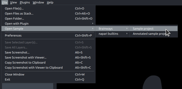
To load one, go to the menu: File -> Open Sample -> Brainways -> Sample project (or Annotated sample project).
Option B: Creating a New Brainways Project#
If you have your own image data, follow these steps:
- Click the
Project -> Newbutton in the right-hand panel. - In the file dialog, select or create a new, empty directory for your project. Brainways will store all project data here.
- The "New Brainways Project" dialog appears. Configure the following:
- Atlas: Select the reference atlas. The whs_sd_rat_39um atlas includes an automatic registration model. Other atlases require manual registration.
- Condition types (Optional): Define experimental variables (e.g.,
treatment,genotype). Separate multiple types with semicolons (e.g.,treatment;genotype). These allow grouping subjects for analysis.
Adding Subjects#
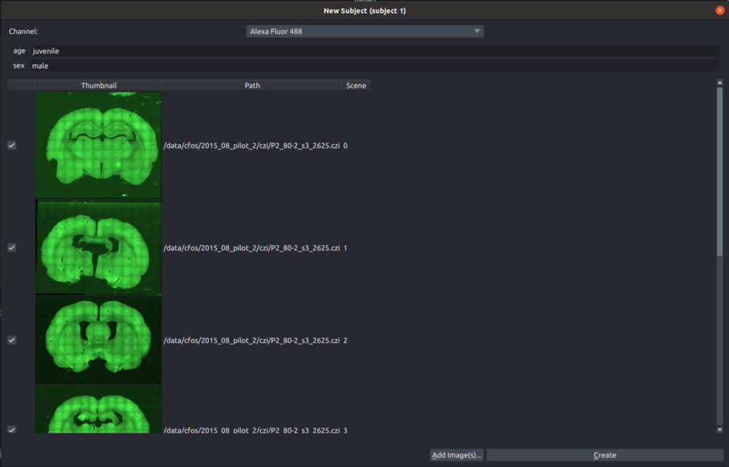
Add each experimental subject (e.g., individual animal) to your project:
- Click the
Add Subjectbutton. - Enter a unique Subject ID.
- If you defined condition types, assign values for this subject (e.g.,
treatment=control,genotype=WT). - Click
Add Image(s)and select all the 2D slice images belonging to this subject (this single brain).- Important: Do not mix images from different brains within one subject.
- If using multi-channel images, select the channel containing the signal you want to quantify (e.g., the fluorescent marker).
- Click
Createto add the subject and their images to the project. - Repeat steps 1-6 for all subjects in your experiment.
4. Working with Brainways: Registration#
After creating a project, the primary task is registering each slice image to the 3D atlas. This involves several steps for each slice.
Best Practices
Before proceeding, review the Best Practices Guide for tips on achieving accurate results.
Keyboard Shortcuts
Most sliders and controls can be adjusted using keyboard shortcuts. Press ? within any registration panel to see the available shortcuts for that step.
The registration process typically involves these stages:
Atlas Registration#
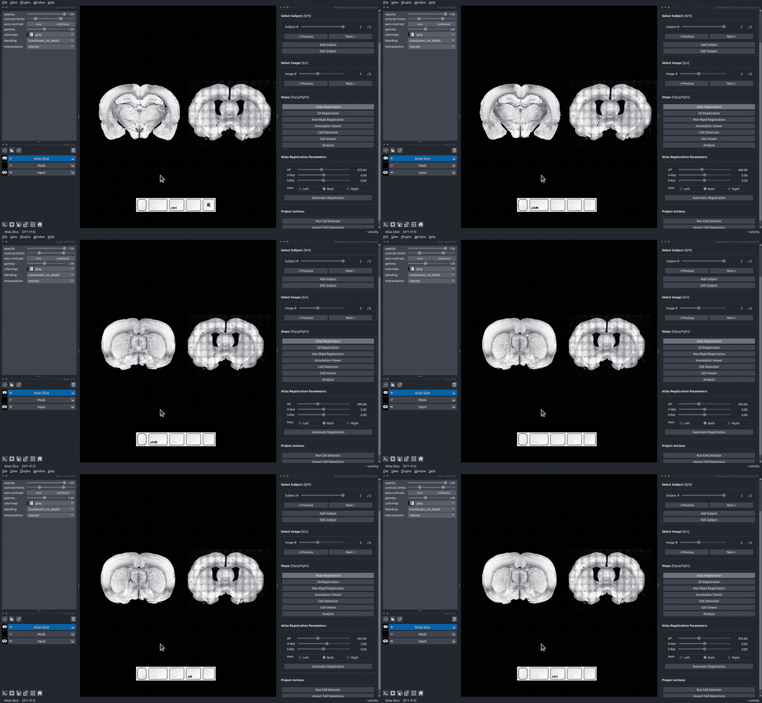
- Goal: Align the slice image (right panel) with the corresponding atlas slice (left panel).
- How: Adjust the sliders in the right panel. If only one hemisphere is present, select it using the "Hem" dropdown.
- Automatic: If an automatic registration model is available for the selected atlas (like whs_sd_rat_39um), it will run automatically when you open an image. You can then refine the result manually if needed.
Rigid Registration (Affine)#
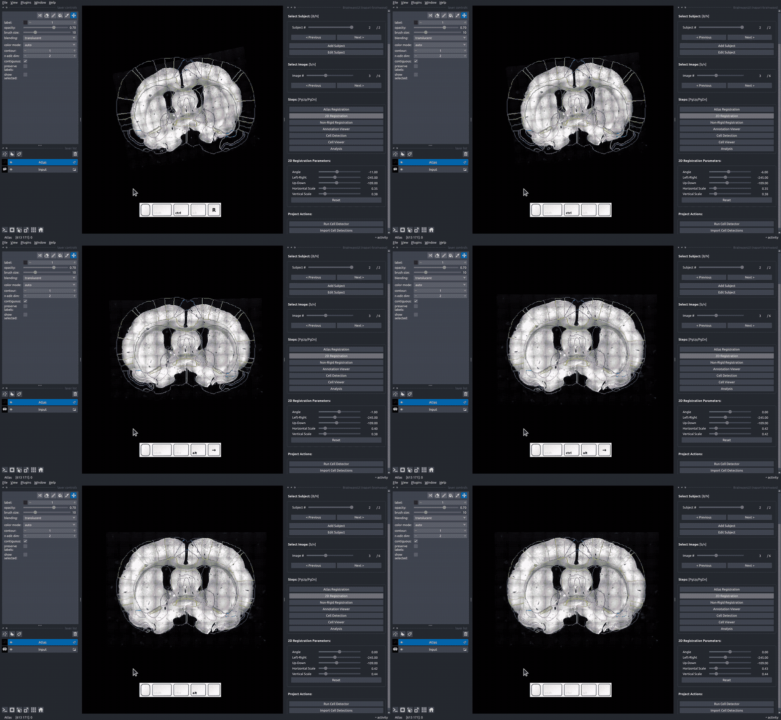
- Goal: Fine-tune the alignment using rotation, scaling, and translation so the slice roughly matches the atlas overlay.
- How: Adjust the sliders in the "Rigid registration" panel.
Non-rigid Registration (Elastic)#
- Goal: Deform the slice image elastically to precisely match the atlas contours, accounting for small anatomical variations.
- How:
- Manual: Drag the blue control points until the underlying image structures align with the atlas overlay.
- Automatic: Click the
Elastixbutton to use the Elastix algorithm for automatic elastic registration (this can take some time).

5. Cell Detection (Optional)#
Brainways uses the StarDist algorithm to detect cells (e.g., labeled neurons) in your images.
Train a Custom Model for Best Results
The default StarDist models may not perform well on all datasets. For optimal accuracy, training a custom StarDist model on your specific experimental data is highly recommended. See the Cell Detection Guide for instructions.
GPU Recommended
As mentioned in the prerequisites, using a GPU significantly speeds up cell detection. Ensure TensorFlow with GPU support is installed if you need faster processing.
Steps:
- Preview (Recommended): Cell detection on full-resolution images can be slow. To test parameters quickly:
- Double-click on a small, representative area in your image to define a preview region.
- Adjust normalization parameters (
Percentile low,Percentile high) in the "Cell detection" panel. - Click
Run on preview. Check the results in the preview area.
- Adjust Parameters:
- Fine-tune normalization parameters based on the preview.
- Unique Settings:
- Check the
uniquebox: The current parameters apply only to this specific image. - Uncheck the
uniquebox: The current parameters become the default for all images in the project (unless overridden by a unique setting).
- Check the
- Run on Full Project: Once satisfied with the parameters (ideally after testing on previews from several images/subjects):
- Click the
Run Cell Detectorbutton. This processes all images in the project, which can take considerable time (potentially hours for large projects).
- Click the

6. Outputs and Analysis#
Once registration is complete (and optionally, cell detection has been run), you can export data and perform analyses.
Exporting Data#
Export Excel with Cell Density per Region#
Generate a spreadsheet summarizing cell counts and densities for each annotated brain region.
- Go to the
Analysissection and clickCalculate results. - Configure the options:
- Min Structure Square Area (μm²): Exclude small regions below this area threshold.
- Cells Per Square Area (μm²): Define the unit area for density calculation (e.g., 10000 for cells/mm²). Raw counts are always included.
- Min/Max Cell Area (μm²): Filter detected cells based on their size (useful for removing noise or artifacts).
- Excel Mode:
Row per Subject: Aggregates data across all slices for each subject.Row per Slice: Provides data for each individual slice.
- Click
OK. The calculation may take some time. - The Excel file will be saved in your project directory.
Export Registered Annotation Masks#
Export the atlas regions mapped onto your slice coordinates. This is useful for analysis in other software.
- Go to the
Analysissection and clickExport Registered Annotation Masks. - Configure the options:
- Output Directory: Choose where to save the mask files.
- Slice Selection: Export masks for the
Current Slice,Current Subject, orAll Subjects. - File Format: Choose
CSV,NPZ(NumPy), orMAT(MATLAB).
- Click
OK. - Files (named after the original images) will be saved in the specified directory.
Performing Analysis#
Brainways offers built-in statistical tools to analyze cell distribution patterns across experimental conditions. Access these via the Analysis panel.
Note
Analysis requires cell detection data. Ensure you have run the cell detector on your project first.
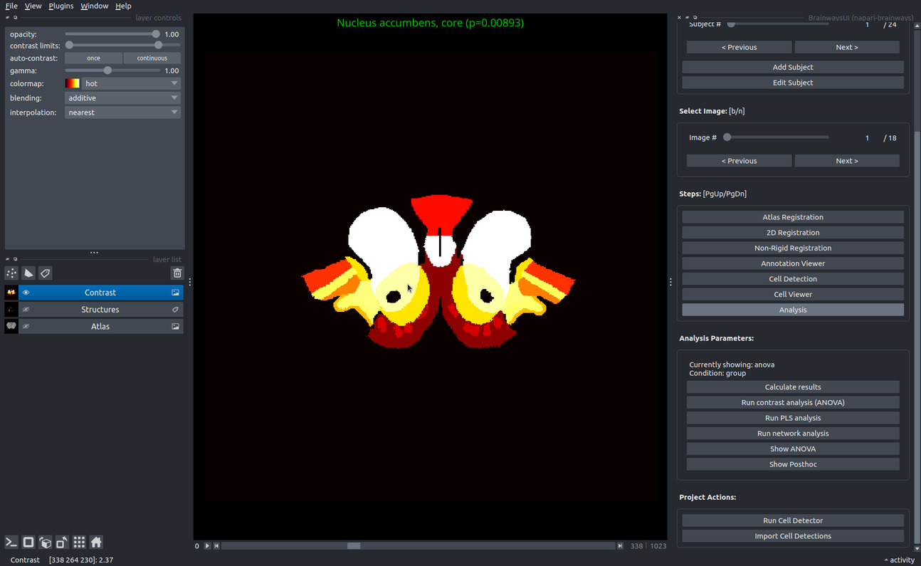
ANOVA Contrast Analysis#
- Purpose: Identify brain regions showing statistically significant differences in cell counts/density between experimental groups defined by your conditions.
- Method: Performs ANOVA on each region, with corrections for multiple comparisons (FDR by default, others available). Post-hoc tests identify specific group differences.
- Output: Results are displayed visually on the atlas and saved to an Excel file:
<PROJECT_DIR>/contrast-<CONDITION>-cells.xlsx. ClickShow Posthocto view pairwise comparisons.
PLS (Partial Least Squares) Contrast Analysis#
- Purpose: A multivariate technique to find patterns of brain region activity that best differentiate experimental conditions.
- Method: Uses the pyls package. Identifies latent variables (LVs) representing condition contrasts and calculates 'saliences' indicating each region's contribution. Significance is assessed via permutation testing and bootstrapping.
- Output: Results (salience plots, LV significance) are saved as PNG and Excel files in
<PROJECT_DIR>/__outputs__/PLS/.
Network Graph Analysis#
- Purpose: Explore functional connectivity by calculating correlations in cell counts between brain regions.
- Method: Creates a graph where nodes are brain regions and edges represent significant Pearson correlations (threshold adjustable, FDR corrected).
- Output: The network graph is exported as a GraphML file (compatible with graph analysis software like Gephi or NetworkX) to
<PROJECT_DIR>/__outputs__/network_graph/.